This page was generated from examples/single.ipynb.

Single-Order Spectrum¶

This will show how to fit a single-order spectrum using our previous setup on some ~mysterious~ IRTF SpeX data. The spectrum is available for download here.

Note: This documentation is not meant to be an exhaustive tour of Starfish’s features, but rather a simple example showing a workflow typical of fitting data.

Preprocessing¶

Normally, you would pre-process your data. This includes loading the fits files, separating out the wavelengths, fluxes, uncertainties, and any masks. In addition, you would need to convert your data into the same units as your emulator. In our case, the PHOENIX emulator uses \(A\) and \(erg/cm^2/s/cm\). For this example, though, I’ve already created a spectrum that you can load directly.

[1]:

%matplotlib inline
import matplotlib.pyplot as plt

plt.style.use("seaborn")

[2]:

from Starfish.spectrum import Spectrum

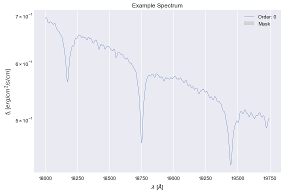
data = Spectrum.load("example_spec.hdf5")

data.plot();

Setting up the model¶

Now we can set up our initial model. We need, at minimum, an emulator, our data, and a set of the library grid parameters. Every extra keyword argument we add is added to our list of parameters. For more information on what parameters are available and what effect they have, see the SpectrumModel documentation.

Some of these parameters are based on guesses or pre-existing knowledge. In particular, if you want to fit log_scale, you should spend some time tuning it by eye, first. We also want our global_cov:log_amp to be reasonable, so pay attention to the \(\sigma\)-contours in the residuals plots, too.

There aren’t any previous in-depth works on this star, so we will start with some values based on the spectral type alone.

[3]:

from Starfish.models import SpectrumModel

model = SpectrumModel(
    "F_SPEX_emu.hdf5",
    data,
    grid_params=[6800, 4.2, 0],
    Av=0,
    global_cov=dict(log_amp=38, log_ls=2),
)
model

[3]:

SpectrumModel
-------------
Data: Example Spectrum
Emulator: F_SPEX_emu
Log Likelihood: None

Parameters
  Av: 0
  global_cov:
    log_amp: 38
    log_ls: 2
  T: 6800
  logg: 4.2
  Z: 0
  log_scale: -0.020519147372786654 (fit)

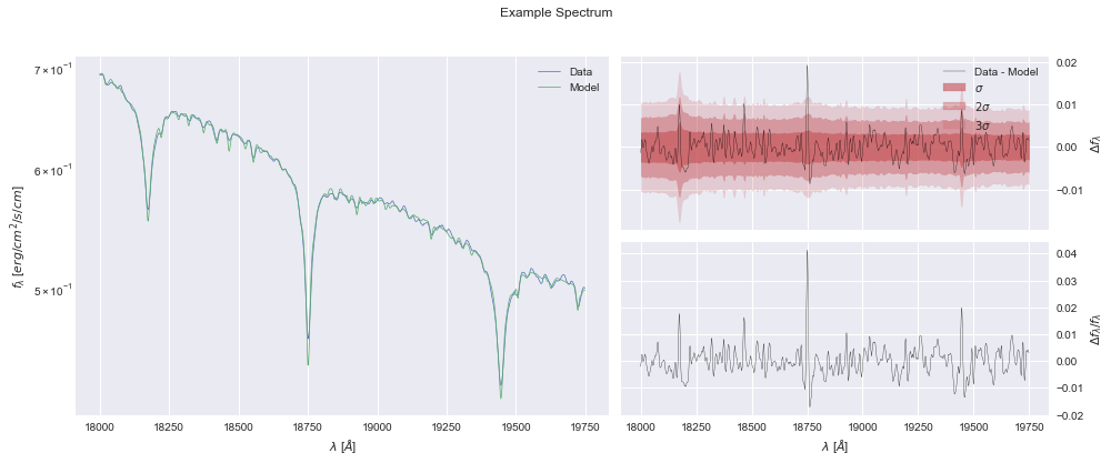
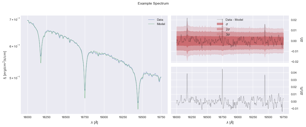
In this plot, we can see the data and model in the left pane, the absolute errors (residuals) along with the diagonal of the covariance matrix as \(\sigma\) contours in the top-right, and the relative errors (residuals / flux) in the bottom-right

[4]:

model.plot();

Numerical Optimization¶

Now lets do a maximum a posteriori (MAP) point estimate for our data.

Here we freeze logg here because the PHOENIX models’ response to logg compared to our data are relatively flat, so we fix the value using the freeze mechanics. This is equivalent to applying a \(\delta\)-function prior.

[5]:

model.freeze("logg")
model.labels  # These are the fittable parameters

[5]:

('Av', 'global_cov:log_amp', 'global_cov:log_ls', 'T', 'Z')

Here we specify some priors using scipy.stats classes. If you have a custom distribution you want to use, create a class and make sure it has a logpdf member function.

[6]:

import scipy.stats as st

priors = {
    "T": st.norm(6800, 100),
    "Z": st.uniform(-0.5, 0.5),
    "Av": st.halfnorm(0, 0.2),
    "global_cov:log_amp": st.norm(38, 1),
    "global_cov:log_ls": st.uniform(0, 10),
}

Using the above priors, we can do our MAP optimization using scipy.optimize.minimze, which is usefully baked into the train method of our model. This should give us a good starting point for our MCMC sampling later.

[7]:

%time model.train(priors)

CPU times: user 5min 1s, sys: 1min 10s, total: 6min 11s
Wall time: 2min 11s

[7]:

 final_simplex: (array([[ 4.35997017e-14,  3.88150634e+01,  4.13042481e+00,
         7.01344658e+03, -3.39321728e-03],
       [ 1.31419453e-13,  3.88150632e+01,  4.13042476e+00,
         7.01344655e+03, -3.39321733e-03],
       [ 1.03637001e-13,  3.88150631e+01,  4.13042471e+00,
         7.01344650e+03, -3.39321746e-03],
       [ 9.47232580e-14,  3.88150633e+01,  4.13042477e+00,
         7.01344654e+03, -3.39321740e-03],
       [ 8.68158683e-14,  3.88150632e+01,  4.13042476e+00,
         7.01344655e+03, -3.39321733e-03],
       [ 6.46583923e-14,  3.88150633e+01,  4.13042476e+00,
         7.01344655e+03, -3.39321734e-03]]), array([-5875.45984265, -5875.45984265, -5875.45984265, -5875.45984265,
       -5875.45984265, -5875.45984265]))
           fun: -5875.4598426469365
       message: 'Optimization terminated successfully.'
          nfev: 960
           nit: 575
        status: 0
       success: True
             x: array([ 4.35997017e-14,  3.88150634e+01,  4.13042481e+00,  7.01344658e+03,
       -3.39321728e-03])

[8]:

model

[8]:

SpectrumModel
-------------
Data: Example Spectrum
Emulator: F_SPEX_emu
Log Likelihood: 5884.738816795258

Parameters
  Av: 4.3599701716468095e-14
  global_cov:
    log_amp: 38.81506339478135
    log_ls: 4.13042481437768
  T: 7013.446581077344
  Z: -0.0033932172800382084
  log_scale: 0.007658916985542291 (fit)

Frozen Parameters
  logg: 4.2

[9]:

model.plot();

[10]:

model.save("example_MAP.toml")

MCMC Sampling¶

Now, we will sample from our model. Note the flexibility we provide with Starfish in order to allow sampler front-end that allows blackbox likelihood methods. In our case, we will continue with emcee, which provides an ensemble sampler. We are using pre-release of version 3.0. This document serves only as an example, and details about emcee’s usage should be sought after in its documentation.

For this basic example, I will freeze both the global and local covariance parameters, so we are only sampling over T, Z, and Av.

[11]:

import emcee

emcee.__version__

[11]:

'3.0.2'

[12]:

model.load("example_MAP.toml")
model.freeze("global_cov")
model.labels

[12]:

('Av', 'T', 'Z')

[13]:

import numpy as np

# Set our walkers and dimensionality
nwalkers = 50
ndim = len(model.labels)

# Initialize gaussian ball for starting point of walkers
scales = {"T": 1, "Av": 0.01, "Z": 0.01}

ball = np.random.randn(nwalkers, ndim)

for i, key in enumerate(model.labels):
    ball[:, i] *= scales[key]
    ball[:, i] += model[key]

[14]:

# our objective to maximize
def log_prob(P, priors):
    model.set_param_vector(P)
    return model.log_likelihood(priors)


# Set up our backend and sampler
backend = emcee.backends.HDFBackend("example_chain.hdf5")
backend.reset(nwalkers, ndim)
sampler = emcee.EnsembleSampler(
    nwalkers, ndim, log_prob, args=(priors,), backend=backend
)

here we start our sampler, and following this example we check every 10 steps for convergence, with a max burn-in of 1000 samples.

Warning: This process can take a long time to finish. In cases with high resolution spectra or fully evaluating each nuisance covariance parameter, we recommend running on a remote machine. A setup I recommend is a remote jupyter server, so you don’t have to create any scripts and can keeping working in notebooks.

[16]:

max_n = 1000

# We'll track how the average autocorrelation time estimate changes
index = 0
autocorr = np.empty(max_n)

# This will be useful to testing convergence
old_tau = np.inf


# Now we'll sample for up to max_n steps
for sample in sampler.sample(ball, iterations=max_n, progress=True):
    # Only check convergence every 10 steps
    if sampler.iteration % 10:
        continue

    # Compute the autocorrelation time so far
    # Using tol=0 means that we'll always get an estimate even
    # if it isn't trustworthy
    tau = sampler.get_autocorr_time(tol=0)
    autocorr[index] = np.mean(tau)
    index += 1
    # skip math if it's just going to yell at us
    if np.isnan(tau).any() or (tau == 0).any():
        continue
    # Check convergence
    converged = np.all(tau * 10 < sampler.iteration)
    converged &= np.all(np.abs(old_tau - tau) / tau < 0.01)
    if converged:
        print(f"Converged at sample {sampler.iteration}")
        break
    old_tau = tau

  2%|▏         | 20/1000 [01:18<1:22:41,  5.06s/it]/Users/miles/.pyenv/versions/3.7.4/Python.framework/Versions/3.7/lib/python3.7/site-packages/ipykernel_launcher.py:28: RuntimeWarning: invalid value encountered in less
 40%|████      | 400/1000 [37:01<55:31,  5.55s/it]

Converged at sample 410

After our model has converged, let’s take a few extra samples to make sure we have clean chains. Remember, we have 50 walkers, so 100 samples ends up becoming 5000 across each chain!

[17]:

sampler.run_mcmc(backend.get_last_sample(), 100, progress=True);

100%|██████████| 100/100 [40:52<00:00, 24.52s/it]

MCMC Chain Analysis¶

Chain analysis is a very broad topic that is mostly out of the scope of this example. For our analysis, we like using ArviZ with a simple corner plot as well.

[18]:

import arviz as az
import corner

print(az.__version__, corner.__version__)

0.11.0 2.1.0

[19]:

reader = emcee.backends.HDFBackend("example_chain.hdf5")
full_data = az.from_emcee(reader, var_names=model.labels)

[20]:

az.plot_trace(full_data);

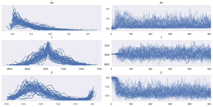
After seeing our full traces, let’s discard and thin some of the burn-in

[21]:

tau = reader.get_autocorr_time(tol=0)
burnin = int(tau.max())
thin = int(0.3 * np.min(tau))
burn_samples = reader.get_chain(discard=burnin, thin=thin)
log_prob_samples = reader.get_log_prob(discard=burnin, thin=thin)
log_prior_samples = reader.get_blobs(discard=burnin, thin=thin)

dd = dict(zip(model.labels, burn_samples.T))
burn_data = az.from_dict(dd)

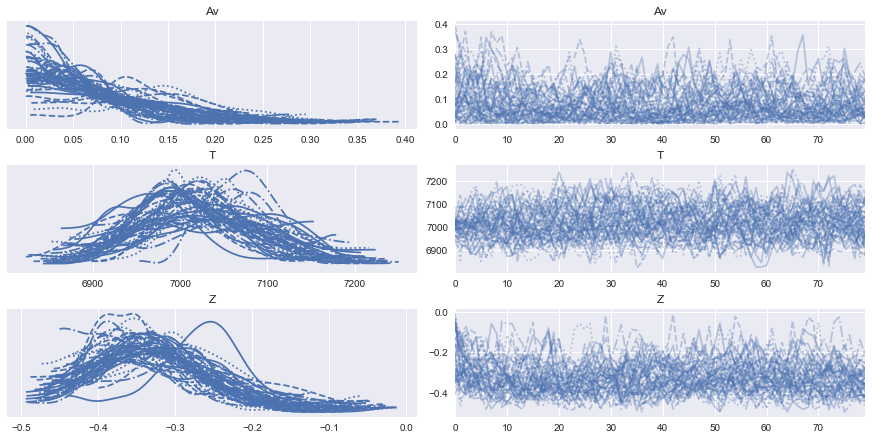
[22]:

az.plot_trace(burn_data);

[23]:

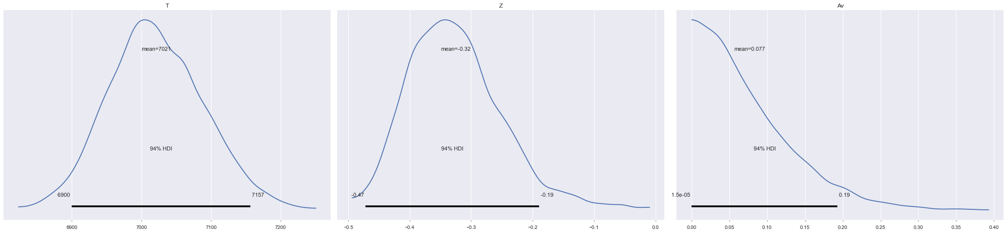
az.summary(burn_data)

[23]:

	mean	sd	hdi_3%	hdi_97%	mcse_mean	mcse_sd	ess_mean	ess_sd	ess_bulk	ess_tail	r_hat
Av	0.077	0.063	0.000	0.193	0.003	0.002	396.0	396.0	437.0	1599.0	1.09
T	7021.219	68.688	6899.632	7156.687	3.331	2.358	425.0	425.0	434.0	1733.0	1.09
Z	-0.325	0.078	-0.472	-0.189	0.003	0.002	514.0	514.0	537.0	1298.0	1.07

[24]:

az.plot_posterior(burn_data, ["T", "Z", "Av"]);

[25]:

# See https://corner.readthedocs.io/en/latest/pages/sigmas.html#a-note-about-sigmas
sigmas = ((1 - np.exp(-0.5)), (1 - np.exp(-2)))
corner.corner(
    burn_samples.reshape((-1, 3)),
    labels=model.labels,
    quantiles=(0.05, 0.16, 0.84, 0.95),
    levels=sigmas,
    show_titles=True,
);

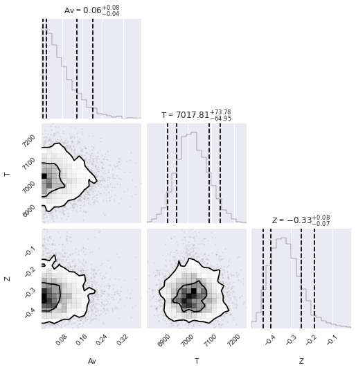
After looking at our posteriors, let’s look at our fit

[26]:

best_fit = dict(az.summary(burn_data)["mean"])
model.set_param_dict(best_fit)
model

[26]:

SpectrumModel
-------------
Data: Example Spectrum
Emulator: F_SPEX_emu
Log Likelihood: 5883.673006463088

Parameters
  Av: 0.077
  T: 7021.219
  Z: -0.325
  log_scale: 0.01143939531892484 (fit)

Frozen Parameters
  logg: 4.2
  global_cov:log_amp: 38.81506339478135
  global_cov:log_ls: 4.13042481437768

[27]:

model.plot();

and finally, we can save our best fit.

[28]:

model.save("example_sampled.toml")

Now, on to the next star!